Original link: https://yufree.cn/cn/2023/10/07/da-pca-paradox/
This is an interesting phenomenon I encountered in my recent research work: there is a set of multidimensional data containing control and control samples. No difference was seen in the principal component analysis, but when performing difference analysis, it was found that there were differences in almost all dimensions. This will form a paradox in interpreting data: if I use principal component analysis to conduct exploratory data analysis, I will think that it is difficult to distinguish the control group from the control group; but if I use single-dimensional difference analysis to compare, even after error Discovery rate controls,differences can be seen in most dimensions. The problem here is that because you show differences in each dimension, the visual differences should be obvious after overall dimensionality reduction. So, are these two sets of data considered to be different or not?
Here I use simulation to reproduce this problem. First, we simulate two sets of data. The control group and the control group both have 100 dimensions, and both have a 1.2-fold mean difference. Each group has 100,000 points:
library(genefilter) # 100个维度np <- rnorm(100,100,100) z <- c() for(i in 1:100){ case <- rnorm(100000,mean = np[i],sd=abs(np[i])*0.1+1) control <- rnorm(100000,mean=np[i]*1.2,sd=abs(np[i])*0.1+1) zt <- c(case,control) z <- cbind(z,zt) }
Let’s take a look at the results of principal component analysis:
pca <- prcomp(z) # 主成分贡献summary(pca)$importance[,c(1:10)]
## PC1 PC2 PC3 PC4 PC5 PC6 ## Standard deviation 143.6913 32.46544 28.8205 27.75735 27.16693 26.65109 ## Proportion of Variance 0.4821 0.02461 0.0194 0.01799 0.01723 0.01659 ## Cumulative Proportion 0.4821 0.50672 0.5261 0.54411 0.56134 0.57793 ## PC7 PC8 PC9 PC10 ## Standard deviation 26.29228 25.84211 25.22661 24.53475 ## Proportion of Variance 0.01614 0.01559 0.01486 0.01406 ## Cumulative Proportion 0.59407 0.60966 0.62452 0.63858
plot(pca$x[,1],pca$x[,2],pch=19,col=c(rep(1,100000),rep(2,100000)))
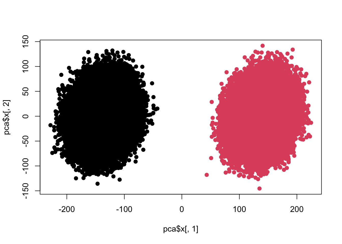
colnames(z) <- 1:ncol(z) re <- colttests(z,factor(c(rep(1,100000),rep(2,100000)))) re$adj <- p.adjust(re$p.value,'BH') sum(re$adj<0.05)
## [1] 100
The difference is obvious. Next we are going to make some changes:
z <- c() for(i in 1:100){ case <- rnorm(100000,mean = np[i],sd=abs(np[i])*0.5+1) control <- rnorm(100000,mean=np[i]*1.2,sd=abs(np[i])*0.5+1) zt <- c(case,control) z <- cbind(z,zt) } pca <- prcomp(z) # 主成分贡献summary(pca)$importance[,c(1:10)]
## PC1 PC2 PC3 PC4 PC5 ## Standard deviation 183.27851 155.32810 139.39841 134.50982 131.62684 ## Proportion of Variance 0.06263 0.04499 0.03623 0.03374 0.03231 ## Cumulative Proportion 0.06263 0.10762 0.14386 0.17759 0.20990 ## PC6 PC7 PC8 PC9 PC10 ## Standard deviation 129.3622 127.52456 124.78930 121.69614 118.3017 ## Proportion of Variance 0.0312 0.03032 0.02904 0.02762 0.0261 ## Cumulative Proportion 0.2411 0.27143 0.30046 0.32808 0.3542
plot(pca$x[,1],pca$x[,2],pch=19,col=c(rep(1,100000),rep(2,100000)))
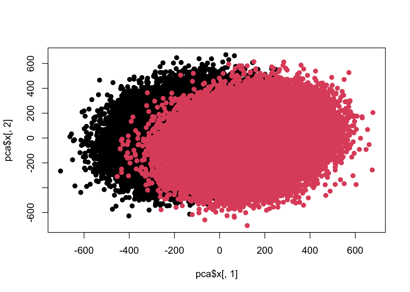
colnames(z) <- 1:ncol(z) re <- colttests(z,factor(c(rep(1,100000),rep(2,100000)))) re$adj <- p.adjust(re$p.value,'BH') sum(re$adj<0.05)
## [1] 100
At present, the differences have begun to merge with each other, so let’s further increase the intensity.
z <- c() for(i in 1:100){ case <- rnorm(100000,mean = np[i],sd=abs(np[i])*0.5+1) control <- rnorm(100000,mean=np[i]*1.2,sd=abs(np[i])*0.5+1) zt <- c(case,control) z <- cbind(z,zt) } pca <- prcomp(z) # 主成分贡献summary(pca)$importance[,c(1:10)]
## PC1 PC2 PC3 PC4 PC5 ## Standard deviation 182.9669 155.40621 139.38457 134.3476 131.78184 ## Proportion of Variance 0.0625 0.04509 0.03627 0.0337 0.03242 ## Cumulative Proportion 0.0625 0.10760 0.14387 0.1776 0.21000 ## PC6 PC7 PC8 PC9 PC10 ## Standard deviation 128.89627 127.35777 124.58692 120.82573 118.27849 ## Proportion of Variance 0.03102 0.03028 0.02898 0.02726 0.02612 ## Cumulative Proportion 0.24102 0.27130 0.30028 0.32754 0.35366
plot(pca$x[,1],pca$x[,2],pch=19,col=c(rep(1,100000),rep(2,100000)))
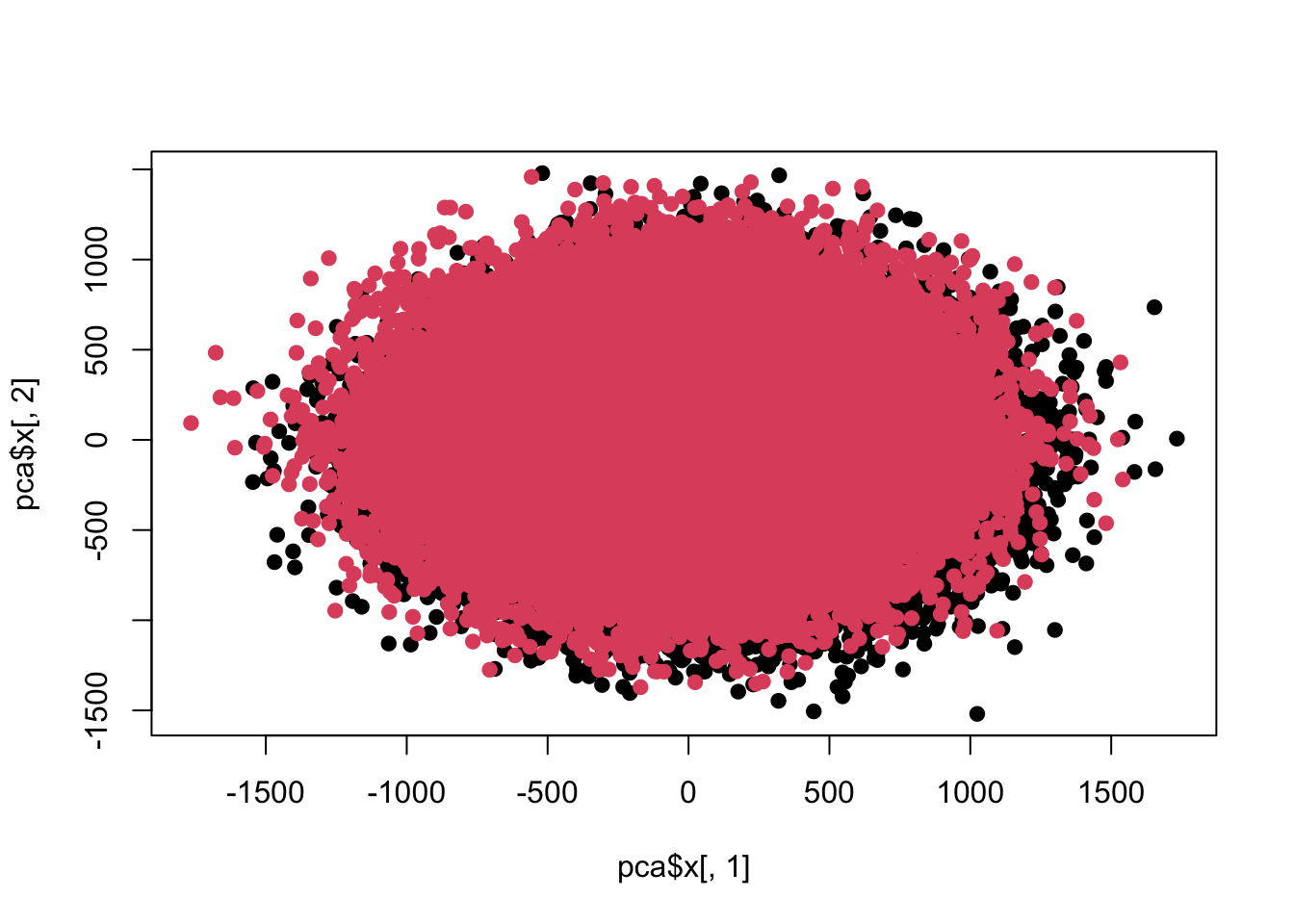
colnames(z) <- 1:ncol(z) re <- colttests(z,factor(c(rep(1,100000),rep(2,100000)))) re$adj <- p.adjust(re$p.value,'BH') sum(re$adj<0.05)
## [1] 100
At present, the difference between the two sets of data is no longer visible in the first two principal components.
In fact, this is not a paradox. The main clue is the variance contribution of the principal component, and the changes I made are also in the relative standard deviation. The first one is 10%, the second one is 50%, and the third one is 120%. . In other words, when the variance in a single dimension has reached the mean level, the first few principal components will not show the original mean difference. In other words, the within-group variance is already greater than the between-group variance, and the first few principal components of the principal component analysis show the direction of the main variance. At this time, it is difficult to see the difference.
Another question is why can we see differences when doing t-test on each dimension? Is this test too sensitive? Here we can try replacing the non-parametric test:
re <- apply(z, 2, function(x) wilcox.test(x~factor(c(rep(1,100000),rep(2,100000))))) pv <- sapply(re, function(x) x$p.value) table(pv)
## pv ## 0 ## 100
The result is very intuitive, there are still differences. So what’s the problem? In fact, it is the nature of the difference itself. This difference is too small and the sample size is too large. As a result, this objectively existing difference will be tested in a large sample. So the ball has been kicked back. Does this weak but existing difference have any physical or scientific significance?
If the difference appears in an irrelevant place, then the difference may not mean much if it exists at all. For example, we compared the thumbnail width of the population of two countries and found that the average thumbnail length of the population in one country was 0.5 mm wider than that of the other country. There is a statistically significant difference, but in a practical sense it is almost zero. However, if this objectively existing difference has practical significance, it will not be easy to find or discover it using exploratory data analysis.
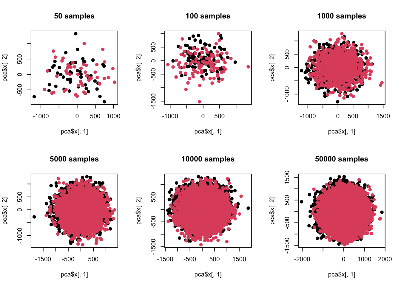
When will this problem occur? That’s when the sample size is particularly large, or now. Let’s now reduce the sample size and take a look:
# 不同样品n <- c(50,100,1000,5000,10000,50000) par(mfrow=c(2,3)) for(t in n){ z <- c() for(i in 1:100){ case <- rnorm(t,mean = np[i],sd=abs(np[i])*1.2+1) control <- rnorm(t,mean=np[i]*1.2,sd=abs(np[i])*1.2+1) zt <- c(case,control) z <- cbind(z,zt) } pca <- prcomp(z) # 主成分贡献print(summary(pca)$importance[,c(1:10)]) plot(pca$x[,1],pca$x[,2],pch=19,col=c(rep(1,t),rep(2,t)),main=paste(t,'samples')) colnames(z) <- 1:ncol(z) re <- colttests(z,factor(c(rep(1,t),rep(2,t)))) re$adj <- p.adjust(re$p.value,'BH') print(sum(re$adj<0.05)) }
## PC1 PC2 PC3 PC4 PC5 PC6 ## Standard deviation 443.89020 418.81034 407.4017 389.1612 384.0458 371.80732 ## Proportion of Variance 0.06506 0.05791 0.0548 0.0500 0.0487 0.04564 ## Cumulative Proportion 0.06506 0.12297 0.1778 0.2278 0.2765 0.32211 ## PC7 PC8 PC9 PC10 ## Standard deviation 347.05778 337.82420 328.59077 322.24252 ## Proportion of Variance 0.03977 0.03768 0.03565 0.03428 ## Cumulative Proportion 0.36188 0.39956 0.43521 0.46949
## [1] 1 ## PC1 PC2 PC3 PC4 PC5 ## Standard deviation 408.68566 384.14060 361.0594 356.38645 338.64842 ## Proportion of Variance 0.05688 0.05026 0.0444 0.04326 0.03906 ## Cumulative Proportion 0.05688 0.10714 0.1515 0.19479 0.23385 ## PC6 PC7 PC8 PC9 PC10 ## Standard deviation 338.4160 321.4941 321.00317 304.24234 297.94794 ## Proportion of Variance 0.0390 0.0352 0.03509 0.03152 0.03023 ## Cumulative Proportion 0.2728 0.3080 0.34315 0.37467 0.40491
## [1] 2 ## PC1 PC2 PC3 PC4 PC5 ## Standard deviation 391.4391 346.68107 335.78486 320.13859 313.30298 ## Proportion of Variance 0.0521 0.04086 0.03834 0.03485 0.03337 ## Cumulative Proportion 0.0521 0.09296 0.13130 0.16614 0.19952 ## PC6 PC7 PC8 PC9 PC10 ## Standard deviation 306.14963 297.96900 294.60451 292.39897 285.56836 ## Proportion of Variance 0.03187 0.03019 0.02951 0.02907 0.02773 ## Cumulative Proportion 0.23139 0.26157 0.29108 0.32015 0.34788
## [1] 90 ## PC1 PC2 PC3 PC4 PC5 ## Standard deviation 385.22172 341.09612 330.20575 322.20941 312.75197 ## Proportion of Variance 0.05025 0.03940 0.03692 0.03516 0.03312 ## Cumulative Proportion 0.05025 0.08965 0.12657 0.16173 0.19485 ## PC6 PC7 PC8 PC9 PC10 ## Standard deviation 308.12069 305.08053 294.47988 287.67776 284.18616 ## Proportion of Variance 0.03215 0.03152 0.02937 0.02802 0.02735 ## Cumulative Proportion 0.22700 0.25852 0.28788 0.31591 0.34325
## [1] 100 ## PC1 PC2 PC3 PC4 PC5 PC6 ## Standard deviation 385.7225 336.8093 328.40787 318.55870 312.53291 306.5494 ## Proportion of Variance 0.0505 0.0385 0.03661 0.03444 0.03315 0.0319 ## Cumulative Proportion 0.0505 0.0890 0.12561 0.16006 0.19321 0.2251 ## PC7 PC8 PC9 PC10 ## Standard deviation 302.60637 293.59629 285.12239 281.76564 ## Proportion of Variance 0.03108 0.02926 0.02759 0.02695 ## Cumulative Proportion 0.25619 0.28544 0.31304 0.33998
## [1] 100 ## PC1 PC2 PC3 PC4 PC5 ## Standard deviation 386.53688 339.35660 326.61421 317.43667 310.75599 ## Proportion of Variance 0.05068 0.03906 0.03618 0.03418 0.03275 ## Cumulative Proportion 0.05068 0.08974 0.12592 0.16010 0.19285 ## PC6 PC7 PC8 PC9 PC10 ## Standard deviation 307.60965 303.10260 294.97926 286.52059 281.26806 ## Proportion of Variance 0.03209 0.03116 0.02951 0.02784 0.02683 ## Cumulative Proportion 0.22494 0.25610 0.28562 0.31346 0.34029
## [1] 100
Here we can see that when the sample is different in a single dimension but the variance is relatively large, when the number of samples exceeds the dimension, there will be a sensitivity difference between difference analysis and principal component analysis. In other words, when the number of samples increases, exploratory data analysis such as principal component analysis can no longer see the preset differences. At the same time, we also noticed that when the sample size is less than the dimension, the power of difference analysis is insufficient, that is, the preset difference cannot be measured at all.
Some people here may wonder whether principal component analysis only considers linear combinations between dimensions. If I change to a nonlinear method, will I still see differences? No problem, let’s continue the simulation:
library(umap) n <- c(50,100,1000,5000) par(mfrow=c(2,2)) for(t in n){ z <- c() for(i in 1:100){ case <- rnorm(t,mean = np[i],sd=abs(np[i])*1.2+1) control <- rnorm(t,mean=np[i]*1.2,sd=abs(np[i])*1.2+1) zt <- c(case,control) z <- cbind(z,zt) } umap <- umap(z) plot(umap$layout,col=c(rep(1,t),rep(2,t)),pch=19,main=paste(t,'samples')) }
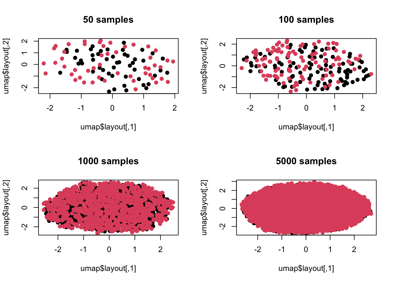
The above is a visualization using umap in manifold analysis. It can be seen that the situation is consistent. After all, the difference during our simulation is not non-linear, so manifold analysis cannot capture this difference.
What I want to say here is that if we rely too much on difference analysis, in the context of large amounts of data, there is a high probability that some objectively existing but weak differences will be detected. These differences can only be found at the mean level, and are very specific to individual differences. It is difficult to see, and it falls into the category where the statistical significance may be greater than the actual significance.
This situation is unlikely to occur in a scenario where the number of samples is smaller than the number of dimensions. The biggest problem in that scenario is the insufficient power of difference analysis, and increasing the sample size is always beneficial. But it can happen when the dimension is much lower than the number of samples. At this time, the law of large numbers has a negative effect, because we can always find differences or patterns, but we lack the means to use professional knowledge to screen the actual significance of the differences.
Obviously, methods such as principal component analysis or cluster analysis are useless at this time. These top-down methods cannot see the heterogeneity in the data at all. However, this may help us filter out some weak differences, and we can only temporarily consider these differences to be insignificant. But the problem you will encounter at this time is the paradox I mentioned at the beginning. It is obvious that the difference analysis has found a lot of differences, but the whole thing seems to be a blur. If you have insufficient data analysis experience, you may not know how to explain it.
This weak difference is essentially a type M error, that is, if the effect is relatively weak, it will have no practical significance if we measure it. Not only in data analysis, this kind of mistake is also very common in our daily lives. For example, financial news reports after the market close every day are often “Affected by so-and-so, the market fell by a few tenths of a percentage point today.” A few tenths of a percentage point is actually a random process and is not affected by someone, but even financial experts have to find an explanation for a lot of noise. What’s even more funny is that after listening to the experts’ advice, the followers of these experts immediately saw the underlying patterns, and then used a sense of superiority to tell others that they were incompetent and could not think of such a far-reaching goal. But the problem is that there is no regularity in the first place, or the uncertainty of the so-called law itself is greater than the certainty. That is, when the variance between samples is large enough, the actual significance of the difference in means between samples is very weak. For example, there is a significant difference in per capita GDP between the two countries, but there is a huge gap between the rich and poor within the two countries. Instead of comparing the per capita GDP, it is better to divide the poor of the two countries into one category and the rich into another category for comparison. The problem discovered at this time Might be more practical.
I generally do not discuss the laws of social sciences. The main reason is that these disciplines have not completed scientific transformation, and their laws are more like a process of self-realization. That is to say, I first construct a set of logically self-consistent theories, and then use the theory to guide practice, how to do it correctly, and use practical actions to prove the feasibility of the theory. But if there are two theories in the same discipline that are logically self-consistent and have been tested by facts, then it is difficult to say which one is the objective law, or that there is no optimal route. This is different from scientific laws. The laws of natural science are relatively unique. It is impossible to agree with both theory A and theory B. In the end, they will be unified by the more general theory C. Many so-called laws in social sciences are actually very subjective academic opinions or cognitive systems. The better ones can be proved through observation and experiments. The extreme ones are simply about logical self-consistency and rolling around in one’s own theoretical circle to keep warm. The golden rule in their eyes may be like what I simulated above, which exists objectively but is actually meaningless, or the classification is not reasonable at all.
Be wary of the differences big data brings.
This article is reproduced from: https://yufree.cn/cn/2023/10/07/da-pca-paradox/
This site is for inclusion only, and the copyright belongs to the original author.