Original link: http://www.nosuchfield.com/2022/06/10/A-brief-look-at-Dynamic-programming/
Dynamic programming is a way to find the optimal solution, and my personal understanding is not very deep. I write randomly, it is a little bit of my own understanding, and criticism is welcome if there is anything wrong. Dynamic programming is a way of deriving the next optimal state from the previous optimal state when transitioning between multiple states, and the previous optimal state is derived from the previous optimal state, so Keep moving forward, and finally we only need to know the initial optimal state. Through the initial optimal state and the logic and method of transition between states, we can obtain the global optimal state. (Does it feel a bit like mathematical induction?)
To give an example of the Fibonacci sequence, the easiest solution is to use recursion.
1 |
def fab (n) : |
A simple analysis shows that in the above example, many numbers are counted repeatedly. For example, fab(3) fab(5) ) is calculated, but fab(3) fab(4) calculated. Therefore, we can use a table to save the already calculated data to avoid repeated calculations
1 |
table = {} |
After changing the strategy, we found that the calculation speed is much faster, which is actually the overlapping sub-problems that dynamic programming needs to avoid. The existence of these overlapping sub-problems leads to a lot of extra computation if brute force exhaustion is used. The solution of dynamic programming is to find the optimal substructure , and finally obtain the optimal solution by continuously performing state transitions between the optimal substructures, and this state transition logic is called the state transition equation .
Observing again, you can know that the calculation of the Fibonacci sequence only depends on the first two values of the current value, so we do not need to use a table to store data, but only need to store two previous value variables.
1 |
def fab (n) : |
From the above, we can know that, in fact, the calculation process of the Fibonacci sequence is a process of using the optimal substructure, state transition equation and initial state to finally obtain the global optimal solution. Let’s look at another example of jumping stairs
There is a stair, you can jump 1 step or 2 steps at a time, ask how many kinds of jumps there are in n steps
The above problem seems impossible to solve, but if you use the above dynamic programming idea to think about it, you can think that the jumping method of jumping n steps is actually equal to the number of jumping methods for jumping n - 1 steps, plus jumping n - 2 The number of jumps per step. Why can you think about it this way, because jumping to the last step may be jumping up a step from the n - 1 step, so in this case, you only need to consider how many ways to jump from the n - 1 step. . Of course, there is another possibility, jumping up two steps from the n - 2 2th step. In this case, you only need to consider the number of jumping methods for the n - 2 steps. Therefore, the jumping method of jumping n steps is actually equal to the sum of the jumping methods of n-1 and n-2 steps, namely
DP[n] = DP[n - 1] + DP[n - 2]
After the transition equation is determined, we only need to determine the initial state (does it feel more like mathematical induction). A simple analysis shows that there are 1 jumping method for jumping 1 step, and 2 jumping methods for jumping 2 steps (2 jumps at a time, or 1 jump at a time and 2 jumps). which is
DP[1] = 1DP[2] = 2
So we can build the following code logic
1 |
def jump (n) : |
The above is a typical dynamic programming problem solving process. Let’s look at another question
Give k coins of denomination, the denominations are c1, c2 … ck, the number of each coin is unlimited, and then give a total amount, ask the minimum number of coins needed to make up this amount, if it is impossible to make up, the algorithm returns – 1
With the above training, we can have a little idea of this question. First, we need to determine the state transition equation, where the state is the total amount , and the state transition is the change in the remaining amount as the amount follows the increase of coins. To know the minimum number of coins for the amount, we only need to know the minimum number of coins for the amount – amount - c . The minimum number of coins for the amount is the minimum number of coins for the amount - c plus 1. But because there are multiple coins, we also need to judge different amount - c , and first get the optimal solution of its preconditions.
We can get its state transition equation
DP[n] = min(DP[n - c1], DP[n - c2] ... DP[n - ck]) + 1
where DP[0] = 0 and DP[负数] = -1 . From this, we can construct the following code logic
1 |
def coin_problem (coins, amount) : |
The above problem is actually a change exchange problem of LeetCode. The above code has exceeded 93% of submissions in LeetCode, and the efficiency is still good.
We are talking about one-dimensional problems above. In fact, dynamic programming often occurs in the form of two-dimensional arrays. Let me look at an example.
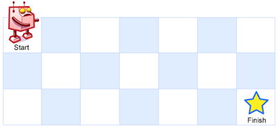
A robot is located in the upper left corner of an mxn grid. The robot can only move to the right or down one grid at a time. How many ways can the robot go to the lower right corner?

Seeing the problem, we can start the analysis. The path the robot takes to the lower right corner can definitely be derived from the path of the previous grid before it reaches the lower right corner. Suppose we mark the grids with coordinates, the horizontal ones are represented by i, and the vertical ones are represented by j, obviously 0 <= i <= m - 1 and 0 <= j <= n - 1 , we can also get the DP transfer equation
DP[i][j] = DP[i - 1][j] + DP[i][j - 1]
In addition, we can find that all the squares in the leftmost column or the uppermost row have only one move. That is, for the leftmost column, the robot can only go down, and for the top row, the robot can only go right, so we can get the initial state
DP[0...m - 1][0] = 1DP[0][0...n - 1] = 1
Get the transition equation and the initial state, then the implementation code is very simple
1 |
def robot_maze (m, n) : |
This is also a topic of LeetCode. My implementation exceeds 91% of the time and 60% of the memory, and the efficiency is still good.
Above we introduced the idea of dynamic programming and the way to solve the problem, the most important of which is the state transition and the determination of the initial state . Through these exercises, we already have some understanding of dynamic programming, and it looks like we are familiar with dynamic programming. But the fact is that the difficulty of dynamic programming is that there are too many variants, and the state transition of some problems is very abstract. When encountering these variants, it may be difficult for us to determine the state design and state transition equations, which can only be improved through continuous practice.
The complete code involved in this article is as follows
1 |
import time |
refer to
How to learn dynamic programming
What is Dynamic Programming? What is the meaning of dynamic programming? – Handsome answer – Knowing
This article is reprinted from: http://www.nosuchfield.com/2022/06/10/A-brief-look-at-Dynamic-programming/
This site is for inclusion only, and the copyright belongs to the original author.