Original link: https://leovan.me/cn/2022/05/rating-and-ranking-algorithms/
In the previous blog ” Is voting fair and reasonable? ” a depressing conclusion has been reached: there is only relative democracy in morality, there is no absolute fairness in institutions . Voting is a ranking of different options or individuals. In voting, we focus more on qualitative conclusions such as relative positions. For example, only the top three students can enter the next session. But sometimes we not only want to know the order of different options, but also want to know the difference between different options. At this time, we need to design a more refined method for quantitative analysis.
Base Scoring and Ranking
direct scoring
From childhood to adulthood, it should be the exam that has been scored the most, 100, 120 or 150. These three numbers should “accompany” us through our youth for more than ten years since the first grade of primary school. The scoring algorithm of the test is simple and easy to distinguish. The whole system sets a total score, and points are added or deducted according to different performances, and the final score is counted as the final score. In general, the grade is a skewed distribution that approximates a normal distribution, as shown in the figure below.
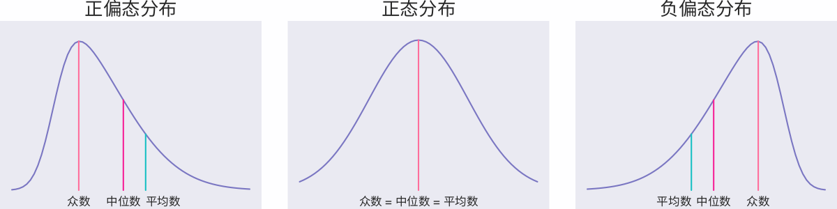
If the scores are approximately normally distributed (as shown in the above picture-middle), it means that the difficulty distribution of this test is relatively balanced; if the overall score distribution is skewed to the left (as shown in the above picture-left), it means that this test is difficult and the students’ scores are generally low. ; If the overall score distribution is skewed to the right (as shown in the figure above – right), it means that this test is relatively easy and the students’ scores are generally high.
In addition, bimodal distribution may also occur, and the steepness and gentleness of the peaks can reflect different problems in the exam, so I will not explain them one by one here. Under normal circumstances, the final score of the test has been able to distinguish the ability of students well, which is why we generally do not do secondary processing of test scores, but use them directly.
weighted score
In real life, different problems and tasks have different levels of difficulty, and in order to ensure “fairness”, we need to assign more points to difficult tasks. This is also reflected in the test paper. Generally speaking, the multiple-choice questions will have lower scores than the multiple-choice questions. After all, if the answer is random, there is still a 50% probability of answering the correct questions correctly, but the multiple-choice questions containing four options are only 25%. % probability to answer correctly.
Weighted scoring balances the difficulty and score of questions and tasks through weights, but the formulation of weights is not an easy process, especially when setting a weight that takes into account multiple dimensions such as objectivity, fairness, and rationality.
Scoring and ranking considering time
Delicious
The simplest and most direct method is to count the number of votes within a certain period of time, and the project with a higher number of votes is a better project. In the old version of Delicious, the top bookmarks leaderboard was based on the number of favorites in the past 60 minutes, and re-counted every 60 minutes.

The advantages of this algorithm are: simple, easy to deploy, and fast to update; the disadvantages are: on the one hand, the ranking changes are not smooth enough, and the content that ranks first in the first hour often plummets in the second hour; on the other hand, there is a lack of automatic Mechanisms to weed out old projects, some popular content may be at the top of the charts for a long time.
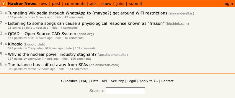
Hacker News
Hacker News is an online community where posts can be posted. Each post has an upward triangle in front of it. If users think the content is good, they can vote with one click. According to the number of votes, the system automatically counts the list of popular articles.
Hacker News uses the following formula for scoring:
$$
Score = \dfrac{P – 1}{\left(T + 2\right)^G}
\label{eq:hacker-news}
$$
Among them, $P$ represents the number of votes for the post, minus $1$ to ignore the voter’s vote; $T$ represents the current time since the post (in hours), plus $2$ to prevent the denominator of the latest post from being too small ; $G$ is the gravity factor, that is, the force that the post ranking is pulled down, the default value is $1.8$.
Under the condition that other conditions remain unchanged, more votes can get higher scores. If you don’t want the gap between “high votes” posts and “low votes” posts to be too large, you can use the formula $\ref{eq:hacker Add an exponent less than $1$ to the numerator of -news}$, for example: $\left(P – 1\right)^{0.8}$. Other things being equal, the score of a post will decrease over time, and after 24 hours, almost all posts will have a score of less than $1$. The effect of the gravity factor on the score is shown in the following figure:
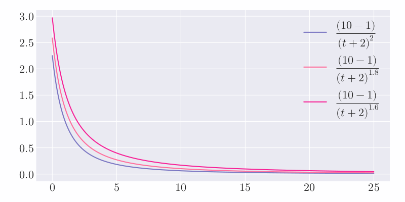
It is not difficult to see that the larger the value of $G$, the steeper the curve and the faster the ranking drop, which means the faster the update speed of the leaderboard.
Unlike Hacker News, each post in Reddit has up and down arrows in front of it, indicating “for” and “against” respectively. Users click to vote, and Reddit calculates the latest hot article rankings based on the voting results.

Reddit’s code for calculating scores can be briefly summarized as follows:
from datetime import datetime, timedelta from math import log epoch = datetime(1970, 1, 1) def epoch_seconds(date): td = date - epoch return td.days * 86400 + td.seconds + (float(td.microseconds) / 1000000) def score(ups, downs): return ups - downs def hot(ups, downs, date): s = score(ups, downs) order = log(max(abs(s), 1), 10) sign = 1 if s > 0 else -1 if s < 0 else 0 seconds = epoch_seconds(date) - 1134028003 return round(order + sign * seconds / 45000, 7)
The score calculation process is roughly as follows:
- Calculate the difference between yes and no votes, that is:
$$
 s = ups - downs
$$ - The median score is calculated using the following formula, namely:
$$
 order = \log_{10} \max\left(\left|s\right|, 1\right)
 $$
Among them, the maximum value of $\left|s\right|$ and $1$ is taken to avoid that $\log_{10}{\left|s\right|}$ cannot be calculated when $s = 0$. The larger the difference between the positive and negative votes, the higher the score. Take the logarithm with the base of $10$, which means that when $s = 10$, this part is $1$, and only when $s = 100$ is $2$, this setting is to reduce the influence of the increase of the difference on the total score degree. - Determine the direction of the fraction, i.e.:
$$
 sign = \begin{cases}
 1 & \text{如果} \ s > 0 \\
 0 & \text{如果} \ s = 0 \\
 -1 & \text{如果} \ s < 0
 \end{cases}
$$ - Calculate the number of seconds since the posting time from December 8, 2005 7:46:43 (the founding time of Reddit?), that is:
$$
 seconds = \text{timestamp}\left(date\right) - 1134028003
$$ - Calculate the final score, which is:
$$
 score = order + sign \times \dfrac{seconds}{45000}
 $$
Divide the time by $45000$ seconds (or 12.5 hours), which means that today’s posts will be about $2$ cents more than yesterday’s posts. If yesterday’s post wants to maintain its previous ranking, the $s$ value needs to be increased by $100$ times.
The Reddit scoring algorithm determines that Reddit is a community for the masses, not a place for radical ideas. Because the difference between upvotes and downvotes is used in the scoring, that is to say, other things being equal, post A has 1 upvote and 0 downvotes; post B has 1000 upvotes and 1000 downvotes, but the discussion Hot Post B has a lower score than Post A.
Stack Overflow
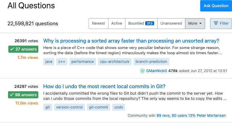
Stack Overflow is the world’s #1 question and answer community for programmers. Users can ask various questions about programming on it and wait for others to answer them; they can vote on the question (for or against) to indicate whether the question is valuable or not; they can also vote on the answer (for or against) , indicating whether the answer is valuable.
On the Stack Overflow page, each question is preceded by three numbers, which are the question’s score, the number of answers, and the number of times the question was viewed.
The calculation formula of the score ranking announced by Jeff Atwood, one of the founders, is as follows:
$$
 \dfrac{4 \times \log_{10}{Q_{views}} + \dfrac{Q_{answers} \times Q_{score}}{5} + \sum \left(A_{scores}\right)}{\left(\left(Q_{age} + 1\right) - \left(\dfrac{Q_{age} - Q_{updated}}{2}\right)\right)^{1.5}}
 $$
in:
-
$4 \times \log_{10}{Q_{views}}$indicates that the more views of the question, the higher the score, and the use of$\log_{10}$to slow down the degree of higher scores as the number of views increases . -
$\dfrac{Q_{answers} \times Q_{score}}{5}$means that the higher the question’s score (difference between upvotes and downvotes), the higher the number of answers and the higher the score. Taking the product form means that a question that is not answered is not a popular question, even if the question itself has a high score. -
$\sum \left(A_{scores}\right)$represents the total score of the question answer. A simple summation is used for the total answer score, but in fact a correct answer outperforms multiple useless answers, and the summation of short answers cannot distinguish the two different situations very well. -
$\left(\left(Q_{age} + 1\right) - \left(\dfrac{Q_{age} - Q_{updated}}{2}\right)\right)^{1.5}$can be rewritten as$\left(\dfrac{Q_{age}}{2} + \dfrac{Q_{updated}}{2} + 1\right)^{1.5}$,$Q_{age}$and$Q_{updated}$represents the time (in hours) of the question and the last answer respectively, that is to say, the longer the question is, and the longer the last answer is, the larger the denominator and the smaller the score.
Stack Overflow’s scoring and ranking algorithm considers engagement (question views and answers), quality (question scores and answer scores), and time (question time and most recent answer).
Scoring and ranking regardless of time
The scoring and ranking methods described above are mostly suitable for time-sensitive information, but for books, movies, etc., where time is not a factor, other methods are needed.
Wilson interval algorithm
Without considering the time, taking the two evaluation methods of “for” and “against” as an example, we usually have two most basic methods to calculate the score. The first is the absolute fraction, that is:
$$
 \text{评分} = \text{赞成票} - \text{反对票}
 $$
But this calculation method sometimes has certain problems, for example: A gets 60 yes votes, 40 no votes; B gets 550 yes votes, 450 no votes. According to the above formula, the score of A is 20, and the score of B is 100, so B is better than A. But in fact, B’s favorable rate is only $\dfrac{550}{550 + 450} = 55\%$ , while A’s favorable rate is $\dfrac{60}{60 + 40} = 60\%$ , So the reality should be that A is better than B.
In this way, we get the second kind of relative score, which is:
$$
 \text{评分} = \dfrac{\text{赞成票}}{\text{赞成票} + \text{反对票}}
 $$
This method is no problem when the total number of votes is relatively large, but it is prone to errors when the total number of votes is relatively small. For example: A gets 2 yes votes, 0 no votes; B gets 100 yes votes, 1 no vote. According to the above formula, the score of A is $100\%$ , and the score of B is $99\%$ . But in fact B should be better than A, because A’s total votes are too small, the data is not very statistically significant.
For this problem, we can abstract:
- Each user’s vote is an independent event.
- Users have only two choices, either to vote for it or to vote against it.
- If the total number of votes is
$n$with$k$upvotes, then the percentage of$p = \dfrac{k}{n}$.
It is not difficult to see that the above process is a binomial experiment. The larger the $p$ , the higher the rating, but the credibility of the $p$ depends on the number of votes, if the number of people is too small, the $p$ is not credible. Therefore, we can adjust the scoring algorithm by calculating the confidence interval of $p$ as follows:
- Calculate the favorable rating for each item.
- Calculate the confidence interval for each positive rating.
- Rank based on the lower bound of the confidence interval.
The essence of the confidence interval is to modify the reliability to make up for the effect of the sample size being too small. If the sample is large enough, it means that it is more credible, and no major correction is needed, so the confidence interval will be narrower, and the lower limit will be larger; if the sample is small, it means that it is not necessarily credible, and a larger , so the confidence interval will be wider and the lower limit will be smaller.
There are various formulas for calculating the confidence interval of the binomial distribution, the most common method of ” normal interval ” is less accurate for small samples. In 1927, the American mathematician Edwin Bidwell Wilson proposed a revised formula, known as the ” Wilson interval “, which solved the problem of accuracy in small samples. Confidence intervals are defined as follows:
$$
 \frac{1}{1+\frac{z^{2}}{n}}\left(\hat{p}+\frac{z^{2}}{2 n}\right) \pm \frac{z}{1+\frac{z^{2}}{n}} \sqrt{\frac{\hat{p}(1-\hat{p})}{n}+\frac{z^{2}}{4 n^{2}}}
 $$
Among them, $\hat{p}$ represents the sample favorable rate, $n$ represents the sample size, and $z$ represents the z statistic of a certain confidence level.
Bayesian averaging algorithm
In some lists, sometimes there are projects with the most votes at the top of the list. It is difficult for new projects or unpopular projects to stand out, and the ranking may be at the bottom for a long time. Taking the world’s largest movie database IMDB as an example, the audience can vote for each movie, with a minimum of 1 point and a maximum of 10 points. The system calculates the average score of each movie based on the voting results.
This raises a question: Are the average scores of popular and unpopular movies really comparable? For example, a Hollywood blockbuster movie may have 10,000 audience votes, and a low-cost literary film may only have 100 audience votes. If the Wilson interval algorithm is used, the score of the latter will be greatly lowered. Is this fair treatment and does it reflect the true quality of the film? In the Top 250 list , the calculation formula of the score and ranking given by IMDB is as follows:
$$
 WR = \dfrac{v}{v + m} R + \dfrac{m}{v + m} C
 $$
Among them, $WR$ is the final weighted score, $R$ is the average votes of the movie users, $v$ is the number of votes for the movie, $m$ is the minimum number of votes for the top 250 movies, and $C$ is Average score for all movies.
As can be seen from the formula, the component $m C$ can be seen as adding $m$ votes for each movie with a rating of $C$ . Then, it is revised according to the movie’s own vote number $v$ and the average vote score $R$ to get the final score. As the number of movie votes increases, the proportion of $\dfrac{v}{v + m} R$ will become larger and larger, and the weighted score will also get closer and closer to the average vote of the movie users.
Writing the formula in a more general form, we have:
$$
 \bar{x}=\frac{C m+\sum_{i=1}^{n} x_{i}}{C+n}
 $$
Among them, $C$ is the scale of the number of voters to be expanded, a reasonable constant can be set according to the total number of voters, $n$ is the number of voters in the current project, $x$ is the value of each vote, and $m$ is the overall average score. This algorithm is called ” Bayesian averaging “. In this formula, $m$ can be regarded as a “prior probability”, and each time a new vote is added, the final score will be revised to make it closer and closer to the true value.
Competition Ratings and Rankings
Kaggle Points
Kaggle is a data modeling and data analysis competition platform. Businesses and researchers publish data on it, and statisticians and data mining experts compete on it to produce the best models. Users participate in Kaggle’s competitions as a team. The team can include only one person. According to the ranking in each competition, points are continuously obtained and used as the final ranking on the Kaggle website.
Early Kaggle points for each match were calculated as follows:
$$
 \left[\dfrac{100000}{N_{\text {teammates }}}\right]\left[\text{Rank}^{-0.75}\right]\left[\log _{10}\left(N_{\text {teams }}\right)\right]\left[\dfrac{2 \text { years - time }}{2 \text { years }}\right]
 $$
In 2015, the new ranking system was adjusted , and the new game points calculation formula was adjusted as follows:
$$
 \left[\dfrac{100000}{\sqrt{N_{\text {teammates }}}}\right]\left[\text{Rank}^{-0.75}\right]\left[\log _{10}\left(1+\log _{10}\left(N_{\text {teams }}\right)\right)\right]\left[e^{-t / 500}\right]
 $$
Among them, $N_{\text{teammates}}$ is the number of team members, $\text{Rank}$ is the competition rank, $N_{\text{teams}}$ is the number of participating teams, and $t$ is from The time elapsed since the end of the game.
The first part can be regarded as base points, the fewer team members, the more base points you will get. From the adjusted document, Kaggle believes that the contribution of each person in teamwork will be greater than $1 / N_{\text {teammates}}$ . In order to encourage teamwork, Kaggle has reduced the basic score penalty for the number of team members.
The second part is to get a coefficient less than or equal to 1 according to the user’s ranking in the competition. The figure below shows the different indices and the difference between $1 / \text{Rank}$ :
![]()
As can be seen from the figure, by adjusting the size of the index, the speed at which the coefficient decreases with the ranking can be controlled. On the whole, Kaggle pays more attention to the top few players. For the top 10 players, the coefficients are all less than $0.2$ , and the difference is not significant.
The third part can be understood as measuring the popularity of the competition (or how easy it is to stand out among the many participating teams) by the number of teams participating. Taking the comparison of 100 and 1000 participating teams as an example, according to the previous calculation formula, this part is:
$$
 \begin{equation}
 \begin{aligned}
 \log_{10} \left(100\right) &= 2 \\
 \log_{10} \left(1000\right) &= 3
 \end{aligned}
 \end{equation}
 $$
But with the increasing popularity of Kaggle’s own competitions, officials believe that winning a 1000-player game does not require $50\%$ more skills than winning a 100-player game, so through the adjusted algorithm, this The scale is adjusted to approximately $25\%$ .
$$
 \begin{equation}
 \begin{aligned}
 \log_{10} \left(\log_{10} \left(100\right) + 1\right) &\approx 0.47 \\
 \log_{10} \left(\log_{10} \left(1000\right) + 1\right) &\approx 0.6
 \end{aligned}
 \end{equation}
 $$
The fourth part is the time decay term, which can be adjusted to a new calculation formula to eliminate the integral cliff caused by setting a 2-year time limit. If no further action is taken by any pair of individuals, the ranking should not change between any pair of individuals. In other words, if the entire Kaggle user base stops participating in competitions, their relative ranking should remain the same over time. The reason for choosing $1 / 500$ is that the old 2 year cliff can be extended to a longer time frame and will never go to 0.
Elo scoring system
Elo Rating System (Elo Rating System) is an evaluation method created by Hungarian-American physicist Arpad Elo to measure the level of various game activities. , football, basketball and other sports. This scoring system is also often used in competitive battle systems of online games.
The Elo scoring system is a statistical-based method for assessing the skill of a chess player. The Elo model originally used a normal distribution, but practice has shown that the performance of chess players is not normally distributed, so the current scoring system usually uses a logistic distribution.
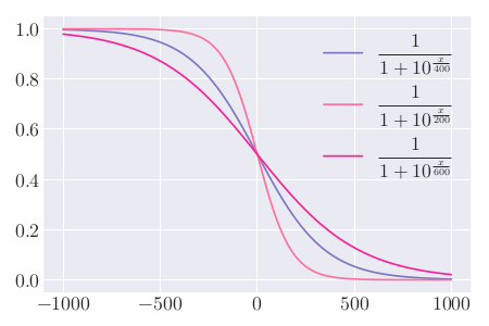
Assuming that the current ratings of players A and B are $R_A$ and $R_B$ R_B$ respectively, then according to the logical distribution, the expected value of A’s winning percentage against B is:
$$
 E_{A}=\frac{1}{1+10^{\left(R_{B}-R_{A}\right) / 400}}
 $$
Similarly, the expected win rate of B against A is:
$$
 E_{B}=\frac{1}{1+10^{\left(R_{A}-R_{B}\right) / 400}}
 $$
If a player’s actual score $S_{A}$ (win 1 point, and 0.5 point, minus 0 point) in the game is different from his expected win rate $E_{A}$ , then his score should be adjusted accordingly adjustment:
$$
 R_{A}^{\prime} = R_{A} + K\left(S_{A}-E_{A}\right)
 $$
In the formula, $R_{A}$ and $R_{A}^{\prime }$ are the scores of the players before and after adjustment, respectively. The value of $K$ $K / 2$ a limit value, which represents theoretically at most one player’s score and loss. In Chess Masters, $K = 16$ ; in most game rules, $K = 32$ . Usually higher-level games have smaller $K$ values, this is done to avoid a few games that can change the rankings of high-end top players. The $400$ in $E_A$ and $E_B$ E_B$ is the value that keeps most players’ points in a standard normal distribution. Under the same $K$ , the larger the value of the denominator position, the smaller the point change value.
Glicko Scoring System
The Glicko Rating System and the Glicko-2 Rating System are one of the methods to assess a player’s technical ability in games such as chess and Go. Invented by Mark Glickman, this method was originally developed for the chess scoring system and has since been widely used as an improved version of the scoring system 1 .
The problem with the Elo scoring system is that there is no way to determine the credibility of player ratings, and the Glicko scoring system improves on that. Assuming that two players A and B with a rating of 1700 each have a match and A wins a match, under the US Chess League’s Elo rating system, player A’s rating will increase by 16, and the corresponding player B’s rating will decrease by 16. But if player A has not played for a long time, but player B plays every week, then player A’s 1700 rating is not very credible in the above case to assess his strength, while player B’s 1700 rating is more reliable. letter.
The main contribution of the Glicko algorithm is Ratings Reliability, or Ratings Deviation. If a player does not have a rating, their rating is usually set to 1500, with a rating bias of 350. The new scoring bias ( $RD$ ) can be calculated using the old scoring bias ( $RD_0$ ):
$$
 RD = \min \left(\sqrt{RD_0^2 + c^2 t}, 350\right)
 $$
Among them, $t$ is the length of time from the last competition to the present (scoring period), and the constant $c$ is calculated according to the technical uncertainty of the players in a specific time period. The calculation method can be based on data analysis or estimation The player’s rating bias will be obtained when it reaches the rating bias of an unrated player. If a player’s rating deviation will reach an uncertainty of 350 within 100 scoring periods, the constant $c$ for a player with a rating deviation of 50 can be obtained by solving $350 = \sqrt{50^2 + 100 c^2}$ , then $c = \sqrt{\left(350^2 - 50^2\right) / 100} \approx 34.6$ .
After $m$ games, the player’s new rating can be calculated by the following equation:
$$
 r=r_{0}+\frac{q}{\frac{1}{RD^{2}}+\frac{1}{d^{2}}} \sum_{i=1}^{m} g\left(R D_{i}\right)\left(s_{i}-E\left(s \mid r_{0}, r_{i}, R D_{i}\right)\right)
 $$
in:
$$
 \begin{equation*}
 \begin{aligned}
 & g\left(R D_{i}\right) = \frac{1}{\sqrt{1+\frac{3 q^{2}\left(R D_{i}^{2}\right)}{\pi^{2}}}} \\
 & E\left(s \mid r, r_{i}, R D_{i}\right) = \frac{1}{1+10\left(\frac{g\left(R D_{i}\right)\left(r_{0}-r_{i}\right)}{-400}\right)} \\
 & q = \frac{\ln (10)}{400}=0.00575646273 \\
 & d^{2} = \frac{1}{q^{2} \sum_{i=1}^{m}\left(g\left(R D_{i}\right)\right)^{2} E\left(s \mid r_{0}, r_{i}, R D_{i}\right)\left(1-E\left(s \mid r_{0}, r_{i}, R D_{i}\right)\right)}
 \end{aligned}
 \end{equation*}
 $$
$r_i$ represents the player’s personal score, and $s_i$ represents the result after each game. A win is $1$ , a draw is $1 / 2$ , and a loss is $0$ .
The function originally used to calculate the scoring deviation should increase the standard deviation value to reflect the increase in the player’s technical uncertainty during a certain non-observation time in the model. Subsequently, the rating bias will be updated after a few games:
$$
 RD^{\prime}=\sqrt{\left(\frac{1}{RD^{2}}+\frac{1}{d^{2}}\right)^{-1}}
 $$
Glicko-2 scoring system
The Glicko-2 algorithm is similar to the original Glicko algorithm, with the addition of a rating volatility $\sigma$ , which measures the expected volatility of a player’s rating based on how erratic the player’s performance is. For example: when a player’s performance remains stable, their rating volatility will be low, and if they have an unusually strong performance after this stable period, their rating volatility will increase by 1 .
The brief steps of the Glicko-2 algorithm are as follows:
Calculate the amount of assistance
In a scoring cycle, the current score of $\mu$ and the score deviation of $\phi$ is compared with $m$ players with the score of $\mu_1, \cdots, \mu_m$ and the score deviation of $\phi_1, \cdots, \phi_m$ players compete, and the points obtained are $s_1, \cdots, s_m$ , we first need to calculate the auxiliary quantities $v$ and $\Delta$ :
$$
 \begin{aligned}
 v &= \left[\sum_{j=1}^{m} g\left(\phi_{j}\right)^{2} E\left(\mu, \mu_{j}, \phi_{j}\right)\left\{s_{j}-E\left(\mu, \mu_{j}, \phi_{j}\right)\right\}\right]^{-1} \\
 \Delta &= v \sum_{j=1}^{m} g\left(\phi_{j}\right)\left\{s_{j}-E\left(\mu, \mu_{j}, \phi_{j}\right)\right\}
 \end{aligned}
 $$
in:
$$
 \begin{equation*}
 \begin{aligned}
 &g(\phi)=\frac{1}{\sqrt{1+3 \phi^{2} / \pi^{2}}}, \\
 &E\left(\mu, \mu_{j}, \phi_{j}\right)=\frac{1}{1+\exp \left\{-g\left(\phi_{j}\right)\left(\mu-\mu_{j}\right)\right\}}
 \end{aligned}
 \end{equation*}
 $$
Determining the new rating volatility
Choose a small constant $\tau$ to limit volatility over time, eg: $\tau = 0.2$ (smaller $\tau$ prevents drastic score changes), for:
$$
 f(x)=\frac{1}{2} \frac{e^{x}\left(\Delta^{2}-\phi^{2}-v^{2}-e^{x}\right)}{\left(\phi^{2}+v+e^{x}\right)^{2}}-\frac{x-\ln \left(\sigma^{2}\right)}{\tau^{2}}
 $$
We need to find the value $A$ that satisfies $f\left(A\right) = 0$ $. An efficient way to solve this problem is to use the Illinois algorithm , once this iterative process is complete, we set the new rated volatility $\sigma'$ as:
$$
 \sigma' = e^{\frac{A}{2}}
 $$
Identify new scoring bias and scoring
Then get the new scoring bias:
$$
 \phi^{\prime} = \dfrac{1}{\sqrt{\dfrac{1}{\phi^{2}+\sigma^{\prime 2}}+\dfrac{1}{v}}}
 $$
and the new rating:
$$
 \mu^{\prime} = \mu+\phi^{\prime 2} \sum_{j=1}^{m} g\left(\phi_{j}\right)\left\{s_{j}-E\left(\mu, \mu_{j}, \phi_{j}\right)\right\}
 $$
It’s important to note that the ratings and rating bias here are not at the same scale as the original Glicko algorithm, and a transformation is required to properly compare the two.
TrueSkill Scoring System
The TrueSkill scoring system is a Bayesian inference-based scoring system developed by Microsoft Research to replace the traditional Elo scoring system and successfully applied to the Xbox Live automatic matchmaking system. The TrueSkill scoring system is an extension of the Glicko scoring system and is primarily used in multiplayer games. The TrueSkill scoring system takes into account the uncertainty of an individual player’s level, taking into account each player’s win rate and possible level fluctuations. When each player has played more games, even if the individual player’s winning rate remains the same, the system will change the player’s rating due to a better understanding of the individual player’s level2 .
In e-sports games, especially when there are multiple players participating in the competition, it is necessary to balance the level of the teams to make the game competition more interesting. Such a contestant ability balance system usually includes the following three modules:
- A module that includes tracking the results of all player matches, recording player abilities.
- A module for pairing contest members.
- A module that announces the abilities of each member of the competition.
Capacity calculation and update
The TrueSkill scoring system is designed for player abilities to overcome the limitations of existing ranking systems and ensure fairness for both sides of the game, and can be used as a ranking system in leagues. The TrueSkill scoring system assumes that the player’s level can be represented by a normal distribution, which can be fully described by two parameters: the mean and the variance. Suppose the Rank value is $R$ , the mean and variance of the two parameters representing the normal distribution of the player’s level are $\mu$ and $\sigma$ , respectively, then the system’s rating for the player, that is, the Rank value is:
$$
 R = \mu - k \times \sigma
 $$
Among them, the larger the value of $k$ , the more conservative the score of the system is.
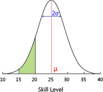
The image above is from the TrueSkill website , the bell curve is the likely distribution of a player’s level, and the green area is the ranking system’s belief that a player’s skill is between level 15 and 20.
The table below shows the changes in $\mu$ and $\sigma$ for 8 novices after participating in an 8-player game.
| Name | ranking | $\mu$ before the game |
$\sigma$ before the game |
$\mu$ after the game |
$\sigma$ after the game |
|---|---|---|---|---|---|
| Alice | 1 | 25 | 8.3 | 36.771 | 5.749 |
| Bob | 2 | 25 | 8.3 | 32.242 | 5.133 |
| Chris | 3 | 25 | 8.3 | 29.074 | 4.943 |
| Darren | 4 | 25 | 8.3 | 26.322 | 4.874 |
| Eve | 5 | 25 | 8.3 | 23.678 | 4.874 |
| Fabien | 6 | 25 | 8.3 | 20.926 | 4.943 |
| George | 7 | 25 | 8.3 | 17.758 | 5.133 |
| Hillary | 8 | 25 | 8.3 | 13.229 | 5.749 |
The 4th Darren and the 5th Eve, their $\sigma$ is the smallest, in other words the system thinks that the possible fluctuations of their abilities are the smallest. That’s because we know the most about them through this game: they won against 3 and 4 people, and they lost against 4 and 3 people. And for the 1st place Alice, we only know that she won 7 people.
Quantitative analysis can first consider the simplest two-player game situation:
$$
 \begin{aligned}
 &\mu_{\text {winner }} \longleftarrow \mu_{\text {winner }}+\frac{\sigma_{\text {winner }}^{2}}{c} * v\left(\frac{\mu_{\text {winner }}-\mu_{\text {loser }}}{c}, \frac{\varepsilon}{c}\right) \\
 &\mu_{\text {loser }} \longleftarrow \mu_{\text {loser }}-\frac{\sigma_{\text {loser }}^{2}}{c} * v\left(\frac{\mu_{\text {winner }}-\mu_{\text {loser }}}{c}, \frac{\varepsilon}{c}\right) \\
 &\sigma_{\text {winner }}^{2} \longleftarrow \sigma_{\text {uninner }}^{2} *\left[1-\frac{\sigma_{\text {winner }}^{2}}{c} * w\left(\frac{\mu_{\text {winner }}-\mu_{\text {loser }}}{c}, \frac{\varepsilon}{c}\right)\right. \\
 &\sigma_{\text {loser }}^{2} \longleftarrow \sigma_{\text {loser }}^{2} *\left[1-\frac{\sigma_{\text {loser }}^{2}}{c} * w\left(\frac{\mu_{\text {winner }}-\mu_{\text {loser }}}{c}, \frac{\varepsilon}{c}\right)\right. \\
 &c^{2}=2 \beta^{2}+\sigma_{\text {winner }}^{2}+\sigma_{\text {loser }}^{2}
 \end{aligned}
 $$
Among them, the coefficient $\beta^2$ represents the average variance of all players, $v$ and $w$ are two complex functions, and $\epsilon$ is the draw parameter. In short, individual players will increase $\mu$ when they win, and decrease $\mu$ when they lose; but regardless of whether they win or lose, $\sigma$ is decreasing, so there may be a situation where the points increase when they lose.
opponent match
Evenly matched opponents make for the best matches, so when automatching opponents, the system tries to match individual players with the closest possible opponents possible. The TrueSkill scoring system uses a function with a value range of $(0, 1)$ to describe whether two people are evenly matched: the closer the result is to 0, the greater the gap, and the closer to 1, the closer the level.
Suppose there are two players A and B, and their parameters are $(\mu_A, \sigma_A)$ and $(\mu_B, \sigma_B)$ , the return value of the function for these two players is:
$$
 e^{-\frac{\left(\mu_{A}-\mu_{B}\right)^{2}}{2 c^{2}}} \sqrt{\frac{2 \beta^{2}}{c^{2}}}
 $$
The value of $c$ is given by the following formula:
$$
 c^{2}=2 \beta^{2}+\mu_{A}^{2}+\mu_{B}^{2}
 $$
If two people have a high probability of being matched together, it is not enough that the average value is close, and the variance needs to be relatively close.
On Xbox Live, the system assigns each player an initial value of $\mu = 25$ , $\sigma = \dfrac{25}{3}$ and $k = 3$ . So the player’s starting Rank value is:
$$
 R=25-3 \frac{25}{3}=0
 $$
Compared with the Elo evaluation system, the advantages of the TrueSkill evaluation system are:
- It is suitable for complex team formation and is more general.
- There is a more complete modeling system, which is easy to expand.
- It inherits the advantages of Bayesian modeling, such as model selection.
This article mainly refers to Ruan Yifeng’s series of articles ” Ranking Algorithms Based on User Voting ” and Qian Wei’s ” Game Ranking Algorithms: Elo, Glicko, TrueSkill “.

This article is reprinted from: https://leovan.me/cn/2022/05/rating-and-ranking-algorithms/
This site is for inclusion only, and the copyright belongs to the original author.